Explainers: Inverse Transform Theorem
This post is my submission to 2022’s Summer of Math Exposition 2 (SoME2), a competition encouraging people all around the world to create expository content on their favourite math topics during the summer. I thoroughly enjoyed learning from the submissions from SoME1, and thought to scrape my spare time together this year to submit something for SoME2.
You can learn more about #SoME2 from Grant Sanderson’s(3B1B) video.
Worlds at our fingertips
Modern day computers are pretty amazing simulation machines.
Here’s an example. Say that I am a Bottle Flipping enthusiast and I am eager to simulate 100 bottle flips. To simulate flipping a bottle 100 times, I could instruct my computer to provide 100 simulations. At a technical level, I am modelling bottle flipping as a binomial distribution, and for my simulation I am generating 100 random variates from that distribution.
Code
  [1] 1 0 1 0 0 0 0 0 1 1 0 0 1 0 0 0 0 0 0 0 0 0 0 0 0 0 0 0 0 1 1 0 0 0 1 0 0
 [38] 0 0 1 1 0 0 0 0 0 0 0 0 0 0 1 1 0 0 0 0 1 1 0 0 0 0 0 0 0 0 1 0 0 1 0 0 0
 [75] 1 0 0 0 0 1 0 0 1 1 0 0 0 0 0 0 0 0 0 0 0 1 0 0 0 0
Yes, 🙄 I know bottle flipping was a trend way back in 2016. I needed a success/failure example and it was either this of “coin flips” which I could not bring myself to use
Or, say I’m a sports fan and my football team scores an average of 1 goal per game. I could simulate the goals scored over 100 games, by modelling the goals scored by my team after a Poisson distribution, and once again, run my simulation by generating 100 random variates from this distribution.
  [1] 0 1 2 1 2 2 0 0 1 2 2 0 1 0 1 3 2 2 1 1 2 1 1 1 1 0 4 3 1 0 0 0 2 1 0 1 0
 [38] 0 2 2 1 0 3 1 3 0 0 0 1 1 2 2 1 2 2 0 2 2 0 0 0 1 0 0 2 1 1 2 2 0 3 0 0 0
 [75] 0 0 0 1 1 2 1 2 0 1 3 1 2 0 0 2 2 0 2 1 0 0 2 2 1 1
You get the gist. From models using a single distribution to ones using complex combinations of distributions, our ability to generate random variates allows us to simulate almost any scenario we can think of!
How random variates are generated
But, how do computers even produce these random variates? Surely, there can’t be a specialised function for every one of the infinite distributions out in the world. It turns out that computers have a very simple solution in the form of two ingredients - a pseudorandom uniform generator and the inverse transform theorem.
A pseudoranom uniform generator is an algorithm that produces random variates from a \(Unif~(0,1)\) distribution, producing uniformly random numbers between 0 and 1. There are many different algorithms that can produce uniform random variates and they are judged on how well they can come close to a perfectly random generator. The assortment of different uniform generators each with their pros and cons are interesting, but that will not be the focus of today’s post. Today, I want to focus on the 2nd ingredient, the inverse transform theorem.
Inverse Transform Theorem
The Inverse Transform Theorem is the backbone behind Inverse Transform Sampling, and is how a uniform distribution is transformed to a diverse range of other distributions.
My biggest challenge when I first encountered this theorem was to grasp the key idea behind its simplicity. Here is the theorem:
Let \(X\) be a continuous random variable with c.d.f \(F(x)\). Then \(F(X) \sim Unif(0,1)\).
And, here’s the equally perplexing simple proof:
Let \(Y = F(X)\) and suppose that \(Y\) has a c.d.f \(G(y)\), then \[G(y) = P(Y \leq y) = P(F(Y) \leq y) \] \[ = P(X \leq F^{-1}(y)) = F(F^{-1}(y)) = y\]
Let me explain the mechanics of the theorem. This theorem simply states that given we have a cumulative density function of a continuous random variable, the inverse of the CDF function will produce a Uniform distribution. While the usage of the theorem reads like a straight forward recipe, I had so many questions about why the theorem works:
- Why is the theorem and proof so simple?
- How could this theorem be universally true for any distribution?
- Why did the theorem introduce the cumulative density function seemingly out of nowhere?
Visual connection
And what I see as a recurring theme amongst SoME submissions, is that for many mathematical concepts that appear hard to understand in written form, we can achieve some clarity by expressing the ideas in visual form. Here is my go at it.
Here are a number of cumulative density functions for an assortment of distributions.
Code
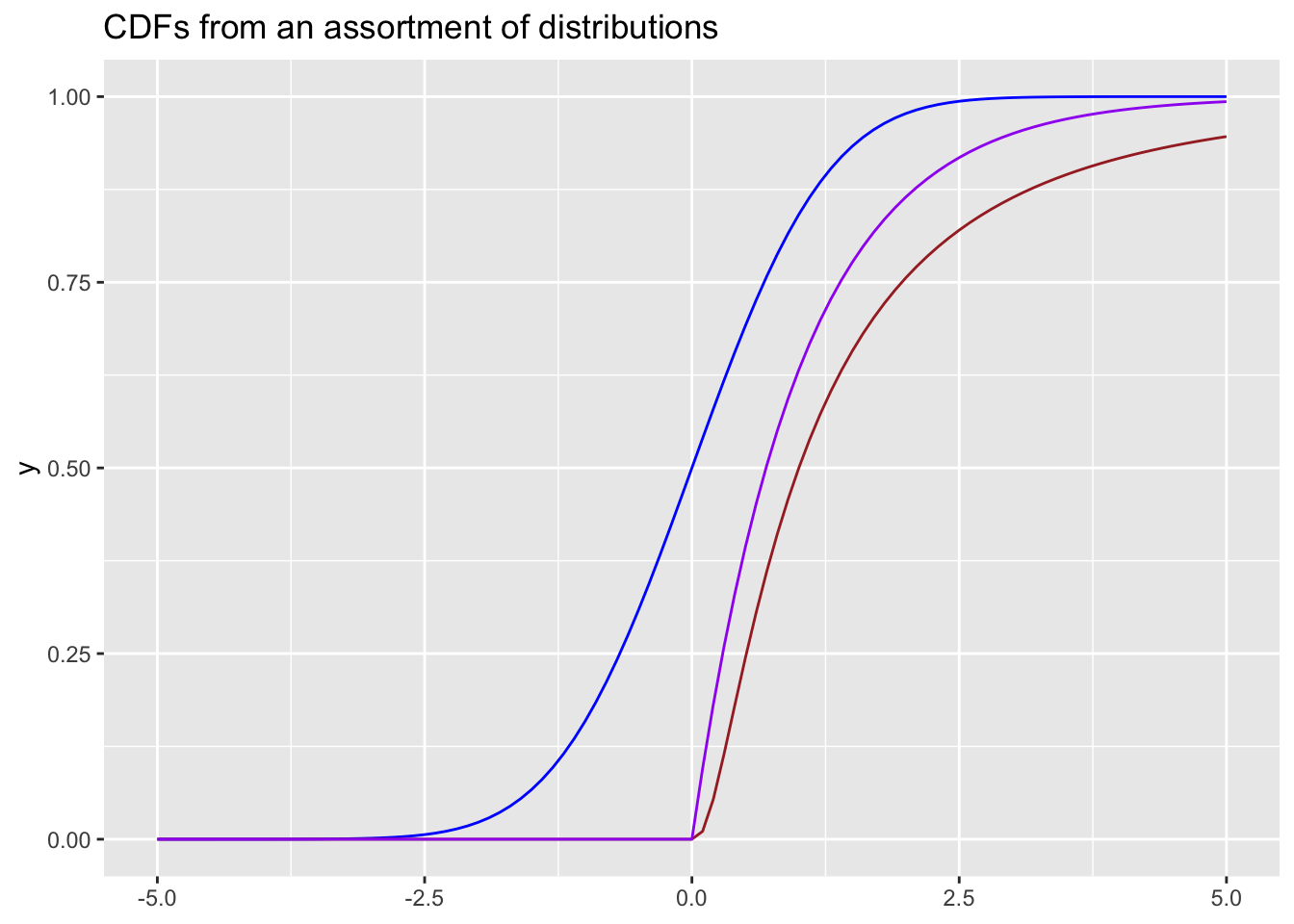
Despite coming in every imaginable shape and size, CDFs for any function have 1 similarity. Their output (y-axis) will always be bound between 0 and 1. This makes a lot of sense when we consider that the CDF is characterised for being a monotonic increasing function. The CDF graphs the probability of \(P(X<x)\), given that the output is a probability, the Y axis will always be bounded between 0 and 1. This property is very useful when we match it back to the \(Unif(0,1)\) distribution. A uniform distribution produces random variates similarly bound between 0 and 1.
The last piece of the puzzle is to understand that just as a function \(F(x)\) can be visually described as a transformation mapping values from the X axis to values on the Y axis, and the inverse of that said function \(F^{-1}(x)\) is simply the inverse transformation mapping values from the Y axis to the X axis.
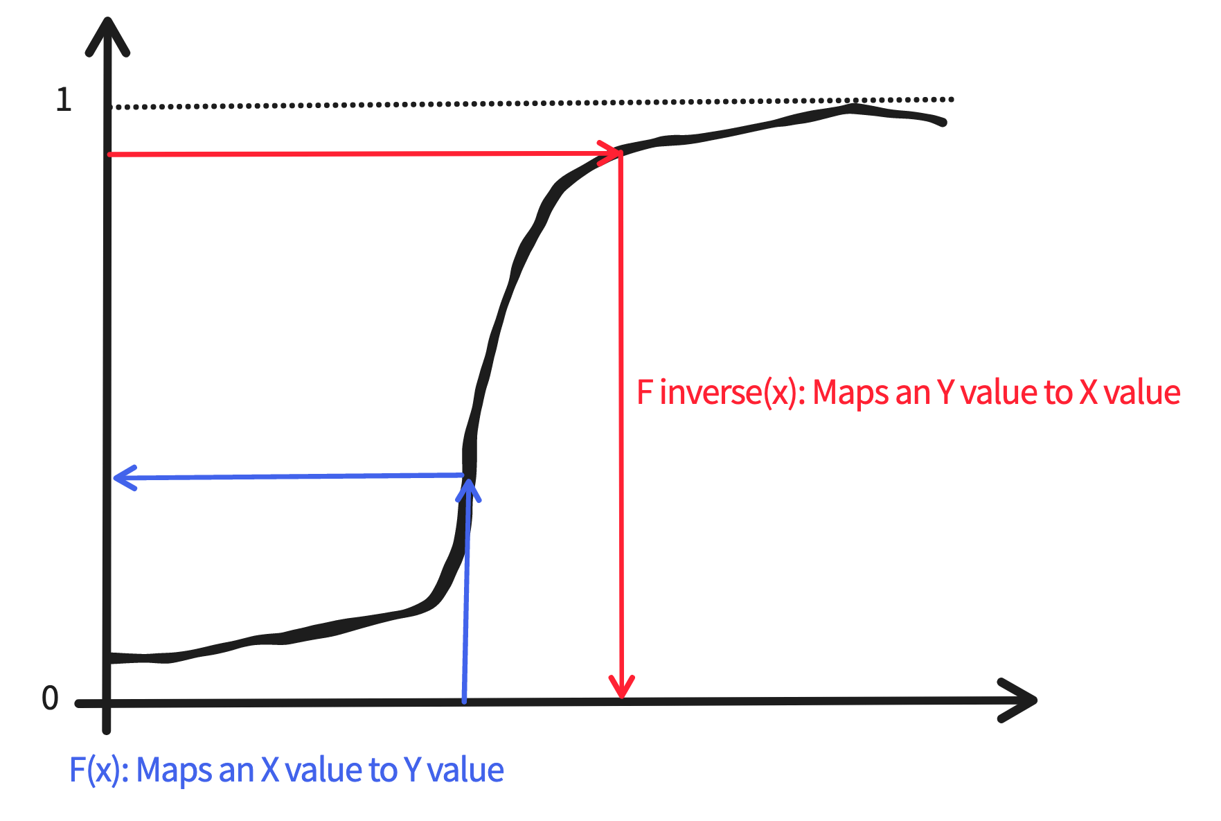
So putting all the pieces together, this is how the Inverse Transform Theorem is put into action:
The \(Unif(0,1)\) distribution produces a random uniform between 0 and 1
This is akin to picking a random point on the Y axis of a CDF for your distribution of interest
The inverse function \(F^{-1}(x)\) maps the random uniform on the Y axis to a value on the X axis
And this X axis value in turn becomes a random variate from your distribution of interest
Conclusion
The Inverse Transform Theorem is a remarkable piece of math that links the uniform distribution to just about any other distribution we could think of. It’s a crucial piece in the machinery of modern machines that enable us to run simulations, and I hope this post helps to share the visual a-ha intuition I experienced when I was learning about this topic.

Appendix
─ Session info ───────────────────────────────────────────────────────────────
 setting  value
 version  R version 4.3.1 (2023-06-16)
 os       macOS Ventura 13.5
 system   x86_64, darwin20
 ui       X11
 language (EN)
 collate  en_US.UTF-8
 ctype    en_US.UTF-8
 tz       Asia/Singapore
 date     2023-08-10
 pandoc   3.1.6 @ /usr/local/bin/ (via rmarkdown)
 quarto   1.3.433

─ Packages ───────────────────────────────────────────────────────────────────
 ! package     * version date (UTC) lib source
 P dplyr       * 1.1.2   2023-04-20 [?] CRAN (R 4.3.0)
 P forcats     * 1.0.0   2023-01-29 [?] CRAN (R 4.3.0)
 P ggplot2     * 3.4.2   2023-04-03 [?] CRAN (R 4.3.0)
 P lubridate   * 1.9.2   2023-02-10 [?] CRAN (R 4.3.0)
 P purrr       * 1.0.1   2023-01-10 [?] CRAN (R 4.3.0)
 P readr       * 2.1.4   2023-02-10 [?] CRAN (R 4.3.0)
   sessioninfo * 1.2.2   2021-12-06 [1] CRAN (R 4.3.0)
 P stringr     * 1.5.0   2022-12-02 [?] CRAN (R 4.3.0)
 P tibble      * 3.2.1   2023-03-20 [?] CRAN (R 4.3.0)
 P tidyr       * 1.3.0   2023-01-24 [?] CRAN (R 4.3.0)
 P tidyverse   * 2.0.0   2023-02-22 [?] CRAN (R 4.3.0)

 [1] /Users/ddanieltan/Code/ddanieltan.com/renv/library/R-4.3/x86_64-apple-darwin20
 [2] /Users/ddanieltan/Library/Caches/org.R-project.R/R/renv/sandbox/R-4.3/x86_64-apple-darwin20/84ba8b13

 P ── Loaded and on-disk path mismatch.

──────────────────────────────────────────────────────────────────────────────
The reward for good work is more work – Tom Sach
Reuse
Citation
@online{tan2022,
  author = {Tan, Daniel},
  title = {Explainers: {Inverse} {Transform} {Theorem}},
  date = {2022-08-08},
  url = {https://www.ddanieltan.com/posts/some2},
  langid = {en}
}